Iceberg Hidden Partitioning and Its Impact on Downstream OLAP Query Rewrites

Iceberg hidden partitioning changes who does the work of making SQL fit a table’s physical layout. The analyst writes filters on real columns, and the engine uses those filters to decide which files to skip. For downstream OLAP workloads, that shift makes partition design, planner behavior, and metadata caches operational concerns. Simple SQL can still lead to a costly scan.

How Hive-style partitioning forces a manual contract between the analyst and the physical layout

Hive-style partitioning exposes storage layout as part of the query contract. A path such as /year=2026/month=07/day=13/ encodes partition values, while the metastore holds separate, explicit partition columns. Filtering a timestamp does not automatically prune directories arranged by a derived date. The analyst must add those partition filters too. A query can therefore express the right business question without giving the engine what it needs to skip irrelevant directories.

That omission is expensive but not necessarily visible. The query still returns correct results when missing partition predicates make it run a full scan. On cloud object storage, recursive directory listing adds metadata latency and can trigger API rate limits at scale. Apache Iceberg’s evolution documentation explains that changing a Hive table from daily to hourly partitioning requires a new table and rewritten downstream queries. The arrangement imposes two burdens. Analysts must write partition-aware SQL, and engineers must rewrite the table to change the scheme.

What hidden partitioning actually does — separating the physical layout from the SQL predicate

Hidden partitioning puts the relationship between columns and storage in table metadata. A partition spec declares a mapping, called a transform, from a source column to a partition value. For example, PARTITIONED BY (month(event_timestamp)) declares that mapping for event_timestamp. The transform is part of the table’s definition. It is not a function that users must add to each query to request pruning.

Iceberg’s built-in transforms include the temporal transforms year, month, day, and hour, as well as bucket(N, col), truncate(W, col), identity, and void. Manifest files record which data files belong to which partitions, so directory names no longer provide that contract. A filter on event_timestamp can benefit from its declared month transform without naming a separate partition column. The engine supplies the missing physical translation. That separation lets BI queries, ETL pipelines, and materializations keep their SQL when the partition scheme changes, although their pruning behavior can change with it.

How the query planner resolves a transform against a filter predicate at plan time

The translation begins when the parser isolates the SQL filter as an expression tree. The planner then reads the partition spec and finds the declared source column and transform, such as month(order_date). For a predicate like order_date >= '2026-05-15', transform projection derives a lower partition bound of 2026-05. This bound shows which partitions could hold matching rows. It does not replace the original filter, because the month partition also contains dates before the requested day.

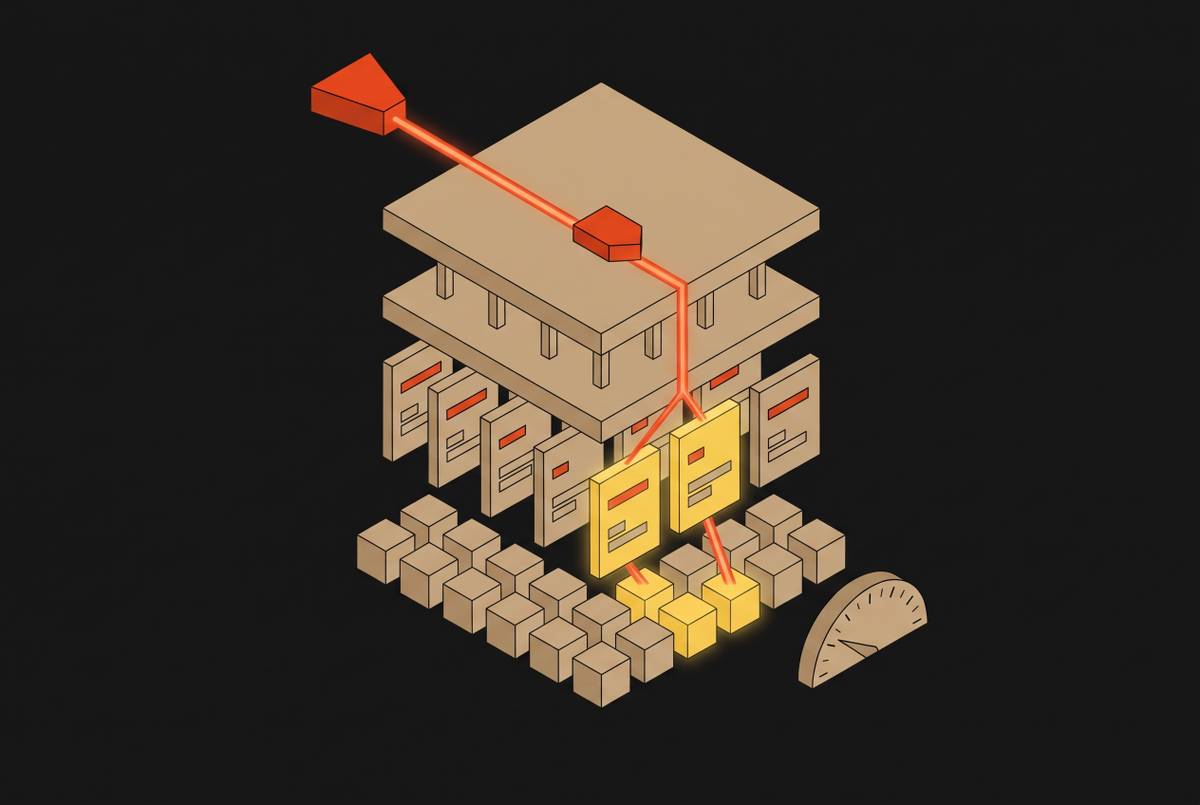
The planner uses that bound at three distinct levels. First, it reads the manifest list, which has minimum and maximum partition-key summaries for each manifest file. A manifest whose range lies entirely outside the bound can be skipped without inspecting its file entries. Second, within surviving manifests, the planner compares each data file’s partition values with the bound. This eliminates non-matching files even when their containing manifest could not be discarded as a whole.

Third, column statistics can rule out more of the files that remain. Per-column minimum and maximum values, held in Iceberg’s column-level metadata or Parquet footers, can rule out files that partition values alone leave eligible. Manifest-list pruning skips groups of file entries, manifest-file pruning skips individual files by partition, and statistics pruning uses column bounds. Where statistics come from footers, accessing them requires only file metadata.

What makes that chain work is the relationship between the predicate and the declared source column. A filter on a different column does not inherit the relationship merely because its values seem equivalent. If transform projection finds no useful bound, partition pruning contributes nothing. If no other pruning path works, the engine scans everything. That is why understanding the source-column match is as important as knowing which transform the table uses.

The conditions under which transform resolution silently fails to prune

A correct result does not show whether pruning worked. Consider WHERE year(event_timestamp) = 2026 AND month(event_timestamp) = 3. Some engines can project those expressions through the declared partition transform, but others cannot. Implicit casts introduce a related uncertainty. If a predicate value cannot be losslessly cast to the required transform domain, the planner may widen the scan to ensure matching rows remain included.

A separate date column creates a more direct mismatch. Querying event_date does not automatically prune a table partitioned by day(event_timestamp), even if the two columns describe the same day. Consequently, SQL that looks partition-aware to its author can still leave the engine with no partition bound.

Mixed-spec tables make the gap harder to spot. Suppose years of data use month(event_time), and a later spec adds identity(customer_region). A region filter can prune partitions for new-spec files, but historical files have no region partition value to test. For that older population, the region condition remains a row-level filter, subject to any other available pruning. None of these missed-pruning paths needs to produce an error or warning, so scan metrics are needed to distinguish a spec mismatch from a simple increase in data volume.

What partition evolution does to the query planner’s job

Iceberg’s evolution documentation specifies that the change is metadata-only, with old files retaining their earlier layout and new files using the new spec. Metadata for the partition versions stays separate. Unlike this mechanism, Delta Lake and Hudi require rewriting existing data to change partitioning. Iceberg avoids that immediate rewrite, but the planner must now interpret more than one layout.

Each manifest records the partition spec used for its files. The planner therefore projects the query filter for each spec used by those files, prunes the files under each spec with its own bounds, and brings together the files that remain. A single SQL predicate can yield different physical filters. In the region example, the new spec supports a region partition test while the old one does not. Stable SQL thus coexists with unequal pruning across the table’s history.

The cost depends on which history queries reach. For workloads focused on recent data, historical partitions are rarely touched, and maintaining two specs adds relatively little planning overhead. Broad analytical queries that filter on several dimensions run into the split more often. Longer evolution histories also give the planner more distinct specs to inspect and apply. Evolution therefore changes future writes and future planning while leaving existing files in their original layout.

When and whether to compact historical files after partition evolution

Rewriting historical files under the new spec can remove that pruning gap, but it requires a separate economic decision. How often do queries reach old data, and how much would the new dimension exclude? If queries with a region filter often span both sets of files, region-based partition pruning cannot skip any old file that passes the time filter. A rewrite can reduce that repeated work. If most requests use recent data, however, the same rewrite spends compute on files that queries rarely touch.

The comparison is between rewrite cost and avoided future reads. When queries often reach old data and a new partition dimension can rule out much of it, compaction can pay for itself within weeks, while history that is rarely read may never be worth the cost. The rewrite cost can rival the original migration. Compaction also offers a second benefit when older files have unsuitable sizes, because right-sizing them can reduce manifest entries and per-file read costs. That benefit belongs in the calculation without making compaction the default answer.

For teams whose workload justifies the rewrite, Iceberg’s rewrite_data_files procedure supports targeted work. Its where predicate selects candidate files by data values, and output-spec-id controls the output partition spec. A historical range can thus select the older files without a rewrite of the whole table. The selection has an important limit. There is no input parameter that filters files directly by their source partition spec ID, so a data-range predicate is not the same thing as a spec-ID selector.

How OLAP engines cache partition statistics and what partition evolution does to those caches

The planner’s work also depends on where its metadata comes from. OLAP engines often cache manifest lists and per-partition statistics in memory so they do not have to read from object storage for every query. That saves planning latency while the cached state fits the table. Statistics for old-spec files remain valid for those files, but they do not supply the missing statistics for new-spec files.

A cache that has not registered the change can apply old-spec bounds to new-spec data or fall back to conservative full-manifest reads. This is a separate concern from weak predicate projection. When projection fails, reading more can still give correct results, but using cached bounds in the wrong way can lead to wrong pruning decisions. Engines that invalidate on snapshot changes handle the transition correctly. Engines using scheduled invalidation can remain stale until their cache TTL expires.

For high-frequency dashboards and iterative AI queries, even a minority of requests taking the broad metadata-read path can increase latency and S3 read costs. The operational response is to treat partition evolution as an engine-level cache invalidation trigger. Teams using several engines against one table need to coordinate that invalidation across every query surface. Changing the table from one engine is not enough. The other engines must also stop planning from stale assumptions.

Remote scan planning may help with this. In this new pattern, the catalog uses transform projection and manifest pruning before it sends file lists back to query engines. That moves responsibility for keeping caches current from engine instances to one server-side component. With correct invalidation still required, it can reduce the reach of a stale-cache window by concentrating the planning state.

Applying these mechanics to real-time analytics workloads — what planner behavior means in practice

Observability pipelines fit these mechanics particularly well because logs, traces, and metrics are append-only, time-ordered, and high-volume, with queries that usually specify a time range. An hour(event_time) partition provides a direct mapping for those filters. Bucketing by a trace or service identifier can also support storage-partitioned joins. For example, logs and spans partitioned by hour and bucketed by trace_id with the same bucket count can support trace reconstruction without a shuffle. Here, the layout serves both filtering and the way related data is joined.

Agentic workloads put additional pressure on the planning path. Agents issue schema exploration and sampling requests as well as analytical queries, so repeated metadata access becomes part of interaction latency. Keeping hot metadata in memory lets the pruning cascade run against cached manifest state rather than repeatedly fetching it from object storage. The benefit becomes sharper at high query concurrency. A useful partition bound still needs an efficient path through the metadata that applies it.

For teams designing these workloads, production query logs should guide partition choices, especially the source columns most often used in filters. Schema and partition evolution make an initial design correctable, but changing it introduces split-spec planning and leaves historical files without the new layout’s full benefit until they are rewritten. Engineers should therefore monitor actual file-pruning rates and manifest read times, and use evolution deliberately. Hidden partitioning removes the analyst’s manual rewrite obligation while leaving the physical contract to be maintained. In production, that responsibility belongs to the engineer who designs the spec, manages its history, and keeps downstream planners aligned with it.