Observability vs Monitoring for High-Volume Event Pipelines

Observability vs Monitoring for High-Volume Event Pipelines.

Why the "is it up?" question stops being enough when pipelines process events at scale

Engineers trained on infrastructure work carry a simple test into everything they build: if the service is running and the dashboard is green, the system is fine. That test holds up when volume is low, because failures at that scale tend to be total and loud. A pipeline goes down, a queue backs up, an alert fires, and someone gets paged within minutes.

Scale changes the shape of failure. Instead of collapsing all at once, pipelines start failing in slices. An event stops firing after a routine release, and the dashboard shows a decline that looks plausible enough that nobody flags it for weeks. Latency creeps up in a single region. Error rates spike only for one customer tier. A pipeline quietly drops a small percentage of events without crossing any threshold that would trigger a page.

None of that appears in red on the monitoring dashboard. The service is up, CPU looks normal, and the queue isn't backing up. Monitoring says everything's fine, because from monitoring's point of view, everything is fine. The problem is that the data moving through the system is wrong, incomplete, or stale, and infrastructure metrics have no way to know that.

Infrastructure failures announce themselves and data failures do the opposite. Infrastructure failures announce themselves: something crashes, something times out, something exceeds a limit. Data failures do the opposite. They hide inside numbers that look reasonable on the surface, and the only way to catch them is to ask a different question than "is it up?"

What monitoring and observability each mean for a data pipeline

Monitoring is rules-based. It tracks metrics you've already decided matter, against thresholds you've already set, and it alerts when one of those known metrics crosses a known line. CPU usage, queue depth, error counts, throughput are the vitals of infrastructure, and monitoring watches them well because you told it in advance what to watch. That's both its strength and its ceiling. It can only catch what someone anticipated.

Observability doesn't require that anticipation. It instruments the environment broadly enough to surface issues nobody wrote a rule for, combining signals and context, tracing and lineage, so an engineer can trace a problem back to its root rather than just getting told a number moved. Applied to a data pipeline specifically, observability means continuously checking the health of the data itself, not just the systems moving it around.

That check breaks into five pillars: freshness, volume, schema, distribution, and lineage. Each one catches something the others miss. Stale data can sail through a throughput check without tripping anything. Schema drift can sail through a volume check the same way. A distribution shift, where the shape of the data itself changes, can pass both a freshness check and a volume check and still be feeding a wrong number into someone's dashboard.

That's the real dividing line between the two disciplines. Monitoring answers "did this known thing break?" Observability answers a harder question: is the data itself trustworthy, right now, whether or not anyone thought to check for this particular failure in advance? The second question doesn't need a pre-written list of what could go wrong. That's exactly what makes it harder to build for, and exactly why it matters more as event volume climbs.

The five failure modes high-volume event pipelines produce that monitoring cannot see

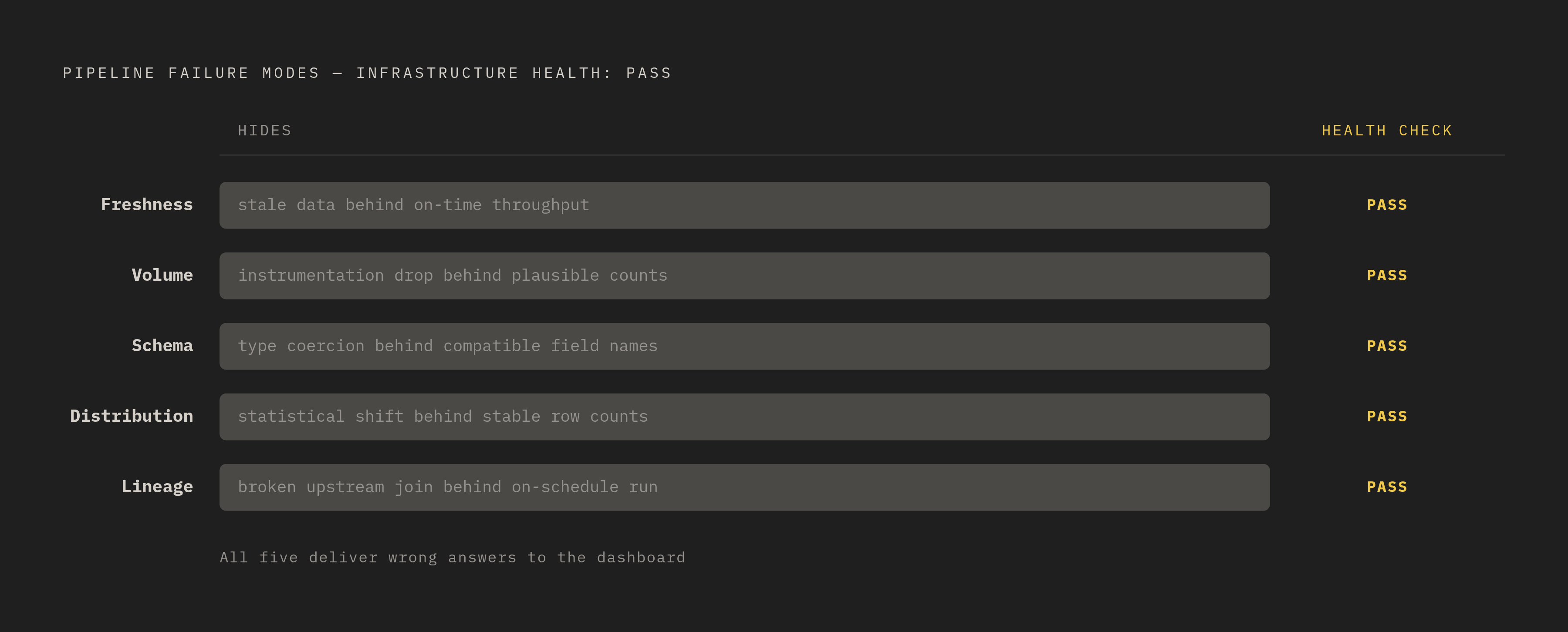
Treat each of the five pillars as a way something breaks, not a feature checklist.

Freshness failure looks fine from the outside: data arrives right on schedule, but what's arriving is a stale snapshot rather than current information. Monitoring sees throughput hitting its expected numbers and calls it a day. It has no concept of "the data that showed up is old."

Volume failure is sneakier at scale, because event counts can drop or spike within a range that still looks plausible. A release ships, some instrumentation quietly stops firing, and the counts settle into a lower but still reasonable-looking pattern that nobody questions.

Schema failure happens when a field changes type or disappears from the payload entirely. Downstream queries don't crash, they just coerce the value or null-fill it and keep going. No infrastructure metric so much as blinks.

Distribution failure is the subtlest of the five. Row counts stay exactly where they should be, but the statistical shape of a column shifts underneath them: a value that was always positive starts going negative, or a field that used to have a few dozen distinct values suddenly has millions.

Lineage failure appears as a dashboard number that looks completely correct, sitting on top of a broken upstream join or a partition that got dropped somewhere in the pipeline. Monitoring has no sense of where a number came from, only whether the process that produced it ran on schedule.

What connects all five is that each one produces data that clears every infrastructure health check while still handing the wrong answer to whoever's reading the dashboard⟦boxc4⟧. And scale makes every one of them harder to spot: as event counts grow, the signal any single anomaly makes gets buried in noise, and at some point nobody can eyeball raw data anymore to sanity-check it. Naming these failure modes in the abstract only goes so far, though. The way they actually show up depends heavily on the database underneath the pipeline, and ClickHouse's architecture, built for speed at scale, creates its own particular blind spots.

How ClickHouse's architecture shapes where data quality problems appear in a pipeline

ClickHouse is columnar and append-only, and that design choice changes what a data quality failure looks like compared to a row-oriented database. Every INSERT lands as its own independent part on disk, and background merges gradually consolidate those parts over time, which is the MergeTree model at its core. That has a direct consequence for anyone trying to catch problems early: a schema anomaly or a distribution shift can sit isolated inside one batch of parts for minutes or hours before merge activity folds it into the rest of the dataset. Whatever's wrong with that batch stays contained, and quiet, until it isn't.

The sparse primary index compounds the problem. ClickHouse doesn't index every row. It indexes in blocks of 8,192 rows, called granules, and for a table holding 8.87 million rows, the resulting index has just 1,083 entries https://clickhouse.com/resources/engineering/clickhouse-query-optimisation-definitive-guide. That's an efficient trade for query speed, since scanning 1,083 entries beats scanning millions of rows. But it means a small batch of malformed events can sit inside a single granule, invisible, until a query happens to read that specific granule. Anomalies smaller than a granule are effectively below the resolution of index-level monitoring.

Some of ClickHouse's most useful features also add a timing wrinkle. Deduplication through ReplacingMergeTree and aggregation through AggregatingMergeTree both happen at merge time, in the background, asynchronously from the original insert. Running a freshness or correctness check before that merge finishes means it reads intermediate, not-yet-final state. Lineage gets murkier too: the authoritative version of a record isn't the one that got inserted, but the one a background merge process eventually produces, and tracking how a record got from A to B means accounting for that extra step.

There's a silver lining buried in all this, though. Part count itself is a usable, leading signal. When the number of active parts in a partition climbs past roughly 100, that's a sign ingestion is outrunning the merge process, and it becomes visible before the resulting data quality problems do, not after. How many teams are actually watching part count as an early warning, versus treating it as background trivia, is worth asking. It's one of the few places where ClickHouse's internals hand you a leading indicator for free.

Schema design decisions that determine whether data quality problems are detectable at all

Fixing a schema mistake in ClickHouse gets expensive fast once a table has real data volume behind it, and there's a second cost that's easy to miss: a schema that hides type information also hides the very signals observability depends on. Get the schema wrong early, and problems that should be visible from day one simply aren't.

The most common version of this mistake is storing a clearly numeric column as a String. It seems harmless. It seems harmless, but it isn't. Strict typing is what makes malformed data detectable in the first place, either failing the insert outright or producing a null or coercion that shows up somewhere in a log. A String column swallows all of that.

Sort key choice affects whether a freshness check runs cheap and fast or turns into a full table scan, even though it looks purely like a performance knob. Putting event_time first in the ORDER BY clause makes a freshness check, asking what the most recent timestamp in the latest partition is, run cheap and fast. Putting user_id first instead turns that same freshness question into a full table scan. The schema isn't neutral here. It either cooperates with the questions observability needs to ask, or it actively resists them.

Partitioning by time earns its keep twice over. It's a performance pattern, sure, but it's also what turns a missing chunk of data into a visible gap in the partition list, rather than a silent zero buried inside a scan of the whole table.

The choice of MergeTree variant carries its own asymmetry too. With ReplacingMergeTree, deduplication doesn't happen until merge time, so row counts taken between merges aren't reliable for volume checks, and any freshness or volume monitoring logic has to build that lag in on purpose. CollapsingMergeTree works differently: it keeps a running log of changes, which is genuinely useful for lineage tracking, but only if whoever's writing the observability queries understands what the sign column is actually doing.

Ingestion patterns that produce observable versus silent failures at high throughput

High-throughput ingestion breaks in ways low-volume ingestion just doesn't. Inconsistent INSERT performance is the first one: batch sizes that vary from insert to insert produce parts of varying size, which throws off merge cadence, which in turn makes part-count-based observability checks unreliable right when they're needed most. The signal gets noisy exactly at the moment things are getting stressed.

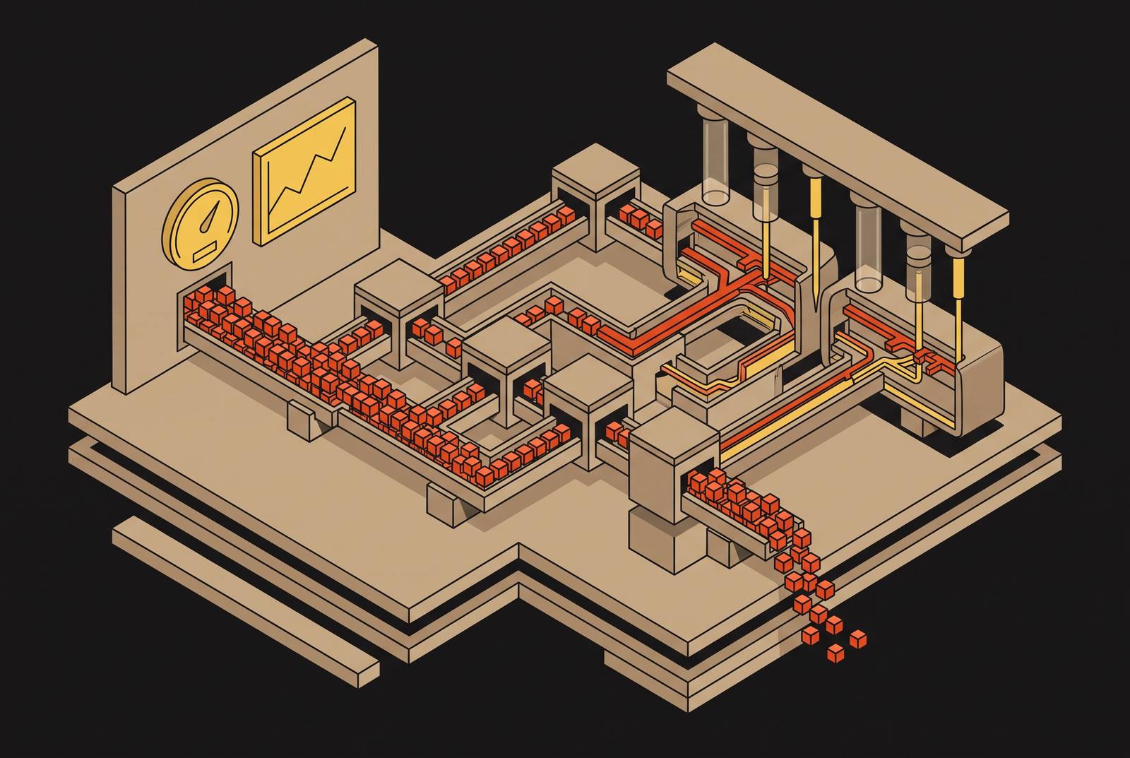
Merge storms are the second pattern. A stream of high-frequency, small inserts piles up small parts faster than merges can consolidate them, and background merge activity starts eating resources that queries need, a problem that's visible in merge performance metrics if anyone's watching. Background merges running past an hour is a documented warning sign worth instrumenting directly.

The KFC architecture pattern introduces additional lineage checkpoints. Every boundary between stages, Kafka offset to Flink processing, Flink output to ClickHouse part, is a place where volume, freshness, and schema can quietly drift out of sync. A schema change that lands in a Kafka topic and gets silently coerced by Flink will look completely fine once it reaches ClickHouse, right up until a distribution check on the ClickHouse side notices the shape of the data has changed. Watching ClickHouse alone misses two-thirds of the pipeline.

Even something as specific as ClickHouse 26.2's move to time-based block flushing changes what a volume check has to assume. Checks built around row-count batches don't automatically translate once flushing switches to time intervals instead of row counts, and low-throughput feeds in particular need their volume logic recalibrated for the new contract.

Materialized views deserve a mention here too, because they can double as an observability layer almost by accident. A materialized view pre-computes aggregates as data lands, and if its running count starts to diverge from a count taken against the raw table, that gap is itself a volume or distribution signal, and an alert should be wired to it rather than discovering it by accident during a debugging session. INSERT latency above 500ms for batch inserts signals partition key issues or merge tree configuration problems (a leading indicator to instrument before it becomes a data quality issue).

What a practical observability layer for a ClickHouse event pipeline covers

Each of the five pillars maps to a specific, checkable pattern inside ClickHouse. Freshness comes down to querying max(event_time); with time-based partitioning already in place, that query stays cheap, and the alert should fire on lag, not on whether the service happens to be up. Volume checks work best when they compare expected counts against a materialized view maintaining a running total at ingest time, rather than hitting the raw table cold every time someone wants an answer.

Schema checks live in system.columns and system.parts, watching for type changes or columns that appeared or vanished without anyone announcing it, and because ClickHouse enforces strict typing, coercions that do slip through tend to leave a trace in the system logs, provided someone's instrumented that trace to be visible. Distribution checks track percentile and cardinality metrics for the columns that matter most, over a rolling window. A column whose p99 value doubles overnight should be flagged even when the row count for that same day looks completely unremarkable.

Lineage checks require instrumenting each stage boundary in the pipeline, Kafka offset, Flink output, ClickHouse part commit, with matching event counts and checksums. Wherever those counts diverge is exactly where data got lost or silently transformed.

Recent ClickHouse releases have started folding some of this into the database itself. Version 26.2 ships with an embedded ClickStack UI, built directly into the ClickHouse binary, for exploring observability data locally. It's meant for development and evaluation, not production; running it in production still means standing up a separate observability system alongside it. Even so, it cuts down on one particular headache: observability infrastructure that itself needs its own monitoring layer to make sure it's working.

Not everything belongs in the observability bucket, and the boundary should be precise. Part count, merge performance, INSERT latency, memory pressure, replication health: these stay squarely in monitoring's territory, because they're known failure modes that a well-set threshold catches reliably. The distinction concerns which layer is watching for health versus watching for trustworthiness, not which layer is more sophisticated. It's about what each one is actually watching: monitoring watches whether the pipeline is healthy, observability watches whether the data flowing through it is trustworthy.

Cadence is the last piece, and it's not the same for every pillar. Freshness and volume checks are cheap enough to run continuously. Distribution and schema checks cost more to run, so they usually land on a schedule instead, and the right interval depends on how fast a given anomaly would actually reach someone downstream before it does damage.

How the database layer itself can carry observability responsibilities rather than outsourcing them

The default architecture treats observability as something bolted on afterward: a separate tool polling the warehouse, comparing counts, firing an alert when something looks off. At low volume, that works fine. At high volume, the observability layer starts generating a query load heavy enough to matter in its own right, and if those checks route through cold storage, they're both slow and expensive, competing with production traffic for the same resources instead of running quietly alongside it.

Keep hot data in memory rather than routing every observability check through object storage like S3. A cache-mesh approach to managed ClickHouse sends observability queries to NVMe storage instead of object storage, which is what makes running freshness and volume checks continuously, rather than on a schedule, actually affordable. That's not a small distinction. Checking freshness once an hour happens because that's what the budget allows, while checking it every few seconds happens because the query barely costs anything.

Full query logging adds another capability that's easy to underrate. Logging every query in complete detail makes lineage reconstruction something done after the fact rather than something planned in advance: "what data did this process read, and when?" becomes answerable without having set up bespoke instrumentation ahead of time to catch that exact question. That matters more as agentic workloads become a bigger share of what hits these pipelines. Agents probe data in parallel, at a frequency and pattern no human analyst would generate, and without full query logging in place, there's no way to audit what they actually touched or whether any of it was already anomalous by the time they read it.

None of this eliminates the operational overhead of running ClickHouse well. Self-hosted deployments still carry a real engineering cost, generally estimated at 10 to 20 percent of an FTE's time just keeping the cluster tuned and healthy https://improvado.io/blog/clickhouse-warehousing-pricing. What shifts is where that effort goes: toward watching data quality directly, instead of only watching whether the infrastructure underneath it happens to be standing up.