Row vs Column Storage Layout Effects on Analytical Query Performance

A dashboard that used to load in half a second starts timing out. The query hasn't changed, the data has just grown, and somewhere a CPU is pegged at full tilt churning through a scan that should have finished already. That split, the same SQL running in milliseconds on one system and minutes on another, isn't about tuning or missing indexes. It comes down to where the bytes physically sit on disk, and what a query has to do to reach them.

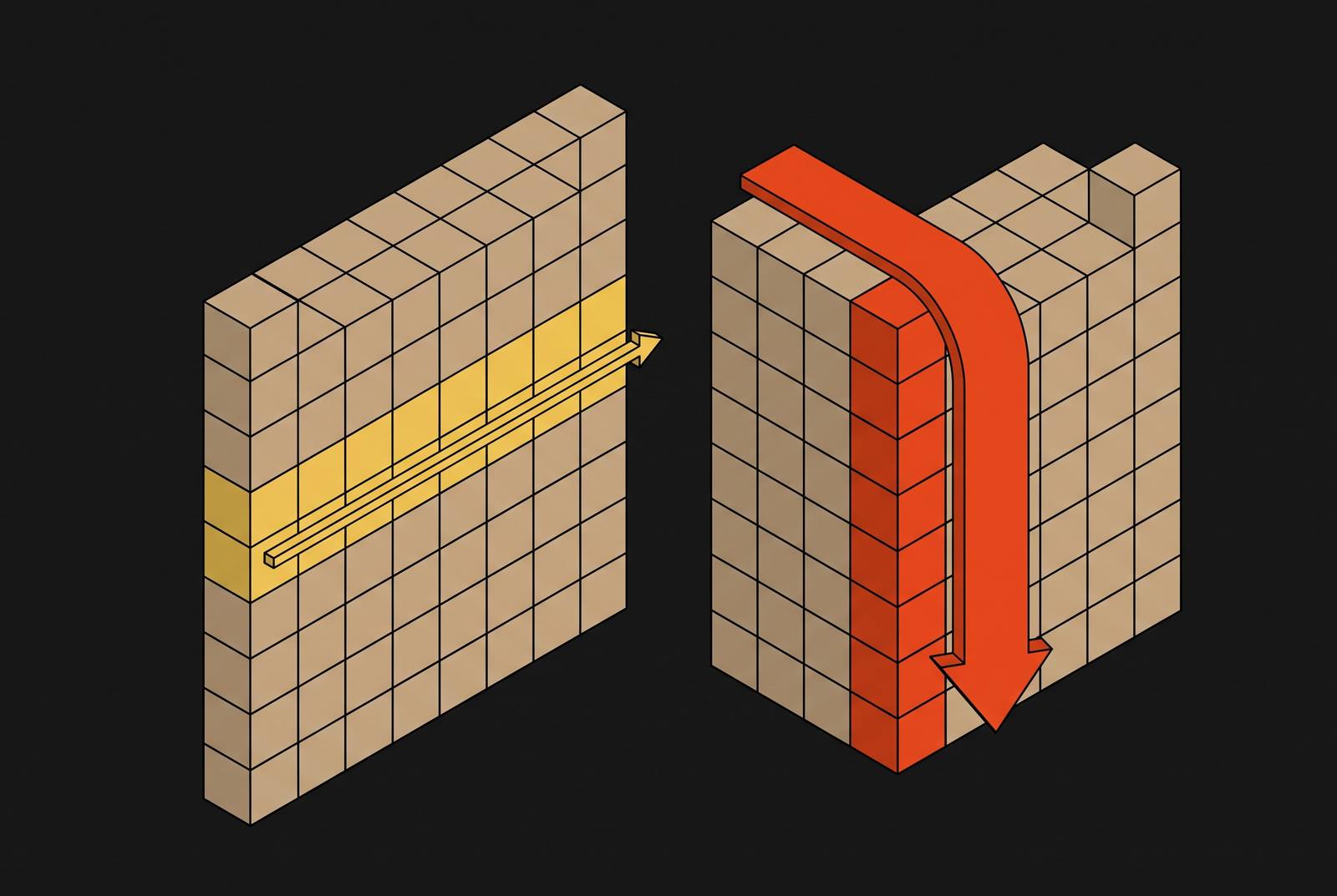
A row store keeps every field of a record next to each other. Ask for one column, and the database still has to read the whole row to get it, dragging along every other field whether the query needs it or not. A columnar store flips that: all the values of a single column sit together, so reading that column means scanning one tight file and skipping the rest. For an analytical query that only touches a handful of fields out of a wide table, that difference in bytes moved is enormous before any other optimization even enters the picture. The rest of this piece is about what happens once it does.

How selective column I/O shrinks the data a query must move

Selective I/O is the first and most direct mechanism, the most straightforward one to understand before anything else gets layered on top. A columnar engine reads only the columns a query actually references, so the bytes it moves from disk to CPU shrink in proportion to how selective the query is. Ask for three columns out of a table with thirty, and the engine reads three column files (plus whatever's needed for filters or joins), not thirty.

A row store can't do this cleanly. Even a query that needs one or two fields still has to pull every row in full, because that's how the data is physically arranged. Every irrelevant field, every column the query never asked for, rides along anyway. There's no index or cache trick that undoes this: it's a consequence of how the bytes are laid out on disk, not a software limitation that can be patched.

Most business intelligence queries touch only a handful of columns out of a much wider table. That's the shape of query selective I/O rewards. The advantage applies to the bulk of analytical workloads almost by default. For most analytical work, though, reduced I/O is only the starting point. What survives that first cut still has to be moved and processed, and that's where compression comes in.

Columnar Compression and Faster Scans

Once a columnar engine has narrowed a scan down to the columns it actually needs, compression shrinks that already-smaller set again. This isn't a separate optimization bolted onto columnar storage after the fact. The layout is what makes the compression possible. Every value in a given column shares the same data type and often a similar range or distribution, so dictionary encoding, run-length encoding, and similar techniques can squeeze that column down far more aggressively than they ever could a row, where types and magnitudes are mixed together in every record.

Row stores pay for that mixing. A column of nothing but dates, or nothing but a repeated category value, compresses in a way a mixed row never will.

The gain compounds directly on top of selective I/O. The engine has already eliminated the columns it doesn't need, and now the columns it does need are compressed, so the actual bytes moved off disk are a fraction of the raw data twice over: once from column pruning, once from compression. Smaller files mean faster scans and lower storage bills, which are really the same physical fact described from two different angles. ObsessionDB's cache-mesh architecture, for instance, keeps hot analytical working sets in distributed NVMe, so the compression gains translate into latency that stays flat as the data grows.

With the data now smaller and denser, the question turns to the CPU. What happens when a processor gets to work on an array of values that are all the same type, packed tightly together, with nothing else mixed in?

SIMD Vectorization and Columnar Layout

Modern CPUs are built to chew through that dense, uniform array fast. Columnar layout produces the memory structure SIMD (single instruction, multiple data) execution needs: a contiguous run of same-type values that loads directly into wide CPU registers, so the processor applies one operation to many values in a single cycle.

Older row-at-a-time processing, sometimes called the Volcano iterator model, works through a query one row at a time: fetch, process a single value, move to the next row, repeat. Vectorized execution instead loads a batch of values, runs the same operation across the whole batch using SIMD instructions, and moves to the next batch. When those batches are sized to fit CPU cache, the engine avoids the branch mispredictions that plague row-at-a-time processing and gets the full benefit of the vectorized instructions.

None of this is available to a row store without extra work. Some engines push this further with late materialization: keeping data in columnar form for as long as possible and only reconstructing full rows after filters and aggregations have already run, which stretches the SIMD benefit across more of the query plan.

Three mechanisms have now been laid out individually: selective I/O, compression, and vectorized execution. None of them, on its own, explains a gap measured in minutes versus milliseconds. What does is what happens when they act together.

How the Three Mechanisms Multiply

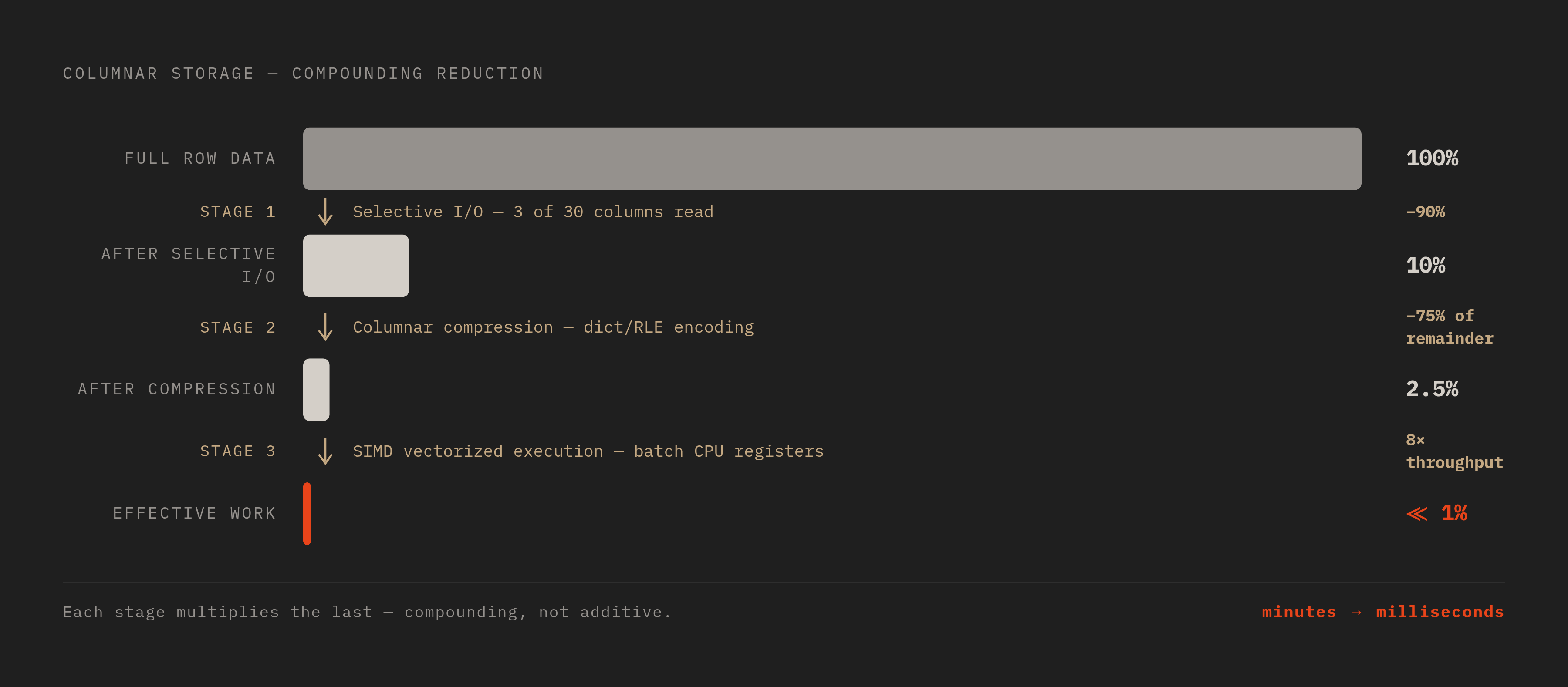
Each mechanism operates on the output of the one before it, not alongside it. That's the structural reason the columnar advantage compounds instead of simply stacking up. Selective I/O narrows a full table down to the columns a query references. Each stage multiplies what the previous stage already saved.

That's also why trying to recreate one mechanism inside a row store never closes the gap. A row store can approximate one link in the chain. It can't replicate the chain.

A wide table with many columns, queried by workloads that only ever touch a handful of them at a time, maximizes all three mechanisms at once: more columns to skip, more uniform data to compress, more dense arrays to vectorize. A narrow table that gets queried column-for-column, where every query touches most of what's there, captures much less of this. The compounding is the actual size of the win.

Block-level pruning as the fourth force that cuts query work before it starts

Before any of those three mechanisms even activate, columnar engines apply one more layer that trims the work further: block-level pruning. Engines store lightweight metadata, min/max value ranges, bloom filters, null counts, alongside every block of data. Before reading a single value out of a block, the engine checks that metadata and decides whether the block could possibly contain anything relevant to the query. If it can't, the block gets skipped.

That skip happens before selective I/O, compression, or SIMD ever touch the block. Pruning multiplies all three mechanisms at once. Pruning doesn't add a fourth independent gain so much as it shrinks the input to the other three before they start.

How well pruning works depends heavily on how the data is sorted on disk. A column whose values track the table's sort order produces tight, narrow min/max ranges per block, and tight ranges mean more blocks get ruled out. A column that's scattered randomly across the sort order produces wide ranges that rarely rule anything out. This is the one mechanism in the whole chain that's most directly shaped by decisions an engineering team actually makes, which sets up the next question naturally: what schema choices put more of this compounding effect to work?

Where Row Layouts Remain Correct

None of this makes columnar storage the right answer everywhere, and being honest about where it isn't is part of understanding why it works where it does. A point-lookup query that needs every field of a single record forces a columnar engine to go fetch each attribute from its own separate column file and reassemble the row. That reassembly cost is the mirror image of the scan efficiency columnar storage delivers elsewhere. On this kind of query it produces a net loss instead of a gain.

Writes tell a similar story. A single-row insert or update in a columnar system means touching multiple separate column files instead of one contiguous row, so columnar engines either absorb that overhead directly or batch writes to amortize it. Either way, high-frequency single-row writes are slower on a columnar system than on a row-oriented one. Row-based systems, by contrast, are built for exactly this kind of CRUD workload. A banking system or a retail order processor handling thousands of small inserts and updates per second benefits from a row store precisely because each operation only touches one or a few rows, and the row layout keeps that touch cheap.

None of this is a flaw in columnar design. It's the direct consequence of an intentional trade-off: optimize for wide scans across few columns, and full-row point access and high-frequency single-row writes pay the cost. Knowing where the line falls is what lets a team pick the right tool instead of assuming one layout wins everywhere, which turns the conversation toward the schema decisions that make the most of columnar storage where it's genuinely the right fit.

Schema design choices that extract more of the compounding gain in practice

Understanding the three mechanisms, plus pruning, isn't academic. It points directly at which schema decisions actually matter, because each of those decisions determines how much of the theoretical compounding gain a real workload gets to keep.

Sort key selection is the clearest example. Putting the column most frequently used in WHERE clauses into the table's sort order tightens the min/max ranges on each block, so block pruning rules out more blocks before any read happens. On an event table, choosing a timestamp as the sort key means a query filtered to a narrow time window can skip every block outside that window before a single column gets decompressed. That pruning gain doesn't stay contained to the pruning stage. It cascades into every mechanism downstream: less I/O, less to decompress, less to vectorize.

Codec choice matters in a similar, concrete way. Dictionary encoding, run-length encoding, and delta encoding each exploit a different pattern in the data, and matching the codec to the column is what captures the full compression multiplier. Apply it instead to a high-cardinality column, like a UUID field where nearly every value is unique, and the encoding has nothing to exploit, so the compression gain that should have compounded with I/O and SIMD gets left on the table.

Materialized views computed at ingestion time address a different part of the chain. Table width and column selectivity round this out: a wide table where most queries touch only a few columns maximizes selective I/O, compression, and SIMD simultaneously, while a narrow table where most queries touch most columns leaves much less of that gain to capture.

ObsessionDB's Architecture at Scale

All three mechanisms, plus block pruning, only deliver their full compounding effect when the hot column data they're operating on is close to the CPU, in memory or on NVMe. Routing every query's compressed column reads through object storage instead brings back the latency the columnar layout was built to eliminate, through the storage layer.

That's the practical issue with managed columnar databases that back every query with a read from S3. The bytes being moved are already small thanks to compression and selective I/O, but the round-trip cost of reaching object storage is paid on every single query, at every level of concurrency, regardless of how few bytes are involved. ObsessionDB addresses this directly with a cache-mesh architecture that keeps hot data on a distributed NVMe cache mesh, so compressed column reads hit local cache. The three mechanisms end up operating at memory bandwidth. Compute and storage stay separated, with S3 backing the system for durability, but the query path itself never has to touch S3 to serve hot data. That separation does its job for reliability and cost without giving up the latency the columnar layout exists to deliver.

The pricing model lines up with that architecture. ObsessionDB charges based on cluster capacity, compute units, rather than per query, so a team running an exploratory analytical workload, or an AI agent issuing speculative queries against a schema, isn't penalized for asking more questions. That's the right economic shape for workloads built around curiosity rather than a fixed, predictable query pattern. For agentic use specifically, ObsessionDB runs agent queries on isolated, read-only compute over the same underlying data, with every query logged in full down to the column, so the concurrency benefits of a columnar engine are available to automated querying without putting production workloads at risk.

ObsessionDB also publishes side-by-side benchmark comparisons on identical workloads, including 2-node cluster runs measured one-to-one against CH Cloud across AWS, GCP, and Azure, with price and latency reported for each provider. That kind of comparison is reproducible by anyone who wants to check it, which is the right basis for a claim about performance, not a marketing line taken on faith.